Are you tired of manually filtering through data in Excel? Do you waste hours trying to find specific information in your vast spreadsheets? Well, the good news is that there are ways to quickly and easily extract data based on specific criteria, allowing you to save time and increase efficiency.
Cara Ambil Data Berdasarkan Nilai Atau Record Yang Sama Di Excel
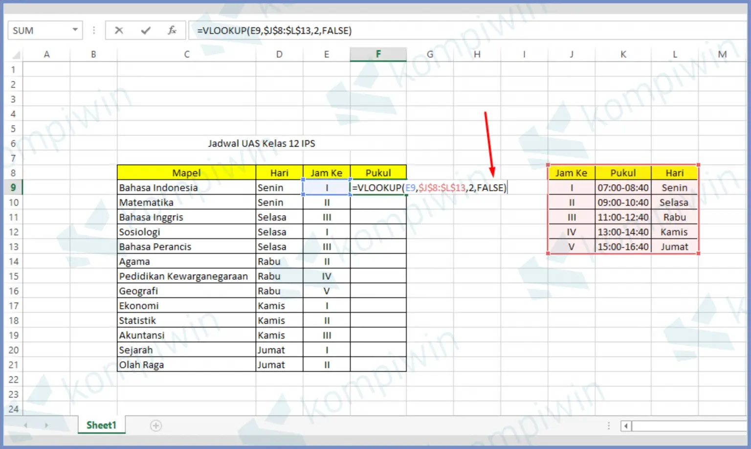
If you’re looking for a way to extract data from one Excel sheet based on specific criteria in another sheet, the “VLOOKUP” function is your friend. This function allows you to search for a specific value in one column of a table, and then return a corresponding value from another column of the same table. Here’s how:
- First, open both the sheet that contains the data you want to extract, and the sheet that contains the criteria you want to use to extract the data.
- Next, select the cell in your extraction sheet where you want the data to appear.
- Then, enter the VLOOKUP function into the formula bar, using the following syntax: =VLOOKUP(lookup_value, table_array, col_index_num, range_lookup)
- Where “lookup_value” is the value you want to search for, “table_array” is the range of cells you want to search within, “col_index_num” is the number of the column that contains the value you want returned, and “range_lookup” is either “TRUE” or “FALSE”, depending on whether you want an exact match or not.
- Press enter, and the corresponding value will appear in your selected cell.
This method can save you a lot of time when dealing with large sets of data. You can simply filter the necessary information using one set of criteria and automatically extract it into another sheet.
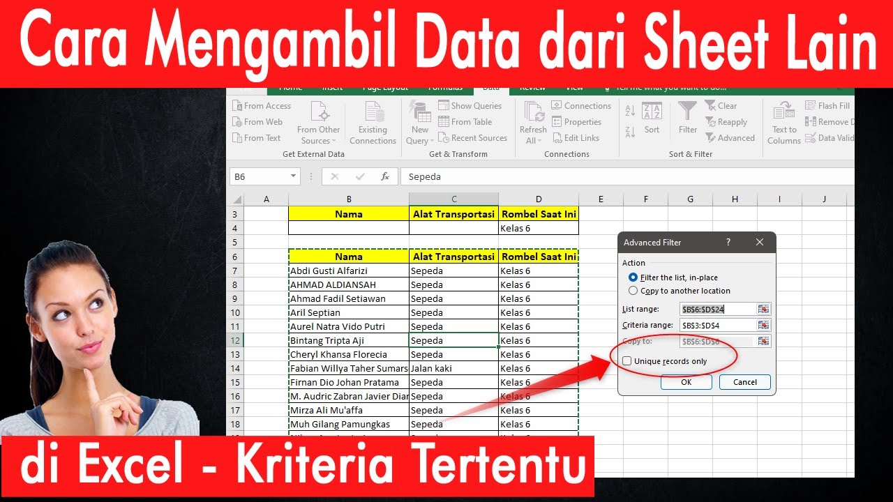
CARA MUDAH MENGAMBIL DATA DARI SHEET LAIN DENGAN KRITERIA TERTENTU DI
If you’re dealing with larger sets of data or multiple sheets within the same workbook, the VLOOKUP method can become tedious and time-consuming. In this case, the most efficient way to extract data is to use a combination of INDEX and MATCH functions.
- First, select the cell in your extraction sheet where you want the data to appear.
- Next, enter the following formula into the formula bar: =INDEX(Table_array, MATCH (Lookup_value, Lookup_array, [Match_type]), Column_number)
- Replace “Table_array” with the range of cells you want to extract data from, “Lookup_value” with the criteria you want to use to extract the data, “Lookup_array” with the range of cells that contains the criteria you want to use, and “Column_number” with the column number of the data you want to extract.
- Press enter, and the corresponding value will appear in your selected cell.
The combination of INDEX and MATCH functions allows you to retrieve data from any column within a range of cells, which provides much more flexibility than the VLOOKUP method. It also eliminates the need to sort your data and can easily be applied to multiple sheets within the same workbook.
FAQ
Q: What if I need to extract data based on multiple criteria?
A: In this case, you can use the combination of INDEX, MATCH, and IF functions. The IF function allows you to specify multiple criteria to be met when retrieving data.
Q: Can I extract data based on specific text within a cell?
A: Yes, you can use the combination of INDEX, MATCH, and SEARCH functions to extract data based on specific text within a cell. The SEARCH function allows you to search for a specific string within a cell and return its position, which can then be used in the INDEX and MATCH functions to extract the necessary data.
These methods of extracting data will allow you to easily filter through large sets of data in Excel and extract the necessary information quickly. Whether you’re dealing with multiple sheets within the same workbook or extracting data based on multiple criteria, these methods will save you time and increase your efficiency.

