Drop-down lists are a valuable tool in Excel, whether you want to control inputs or make data entry more efficient. By creating dynamic lists that are easy to update and maintain, you can streamline your workflows and make better use of your time. In this article, we will walk you through the steps to create drop-down lists in Excel, and offer tips and tricks to help make your work smoother and more efficient.
Creating a Basic Dropdown List
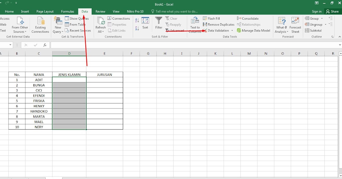
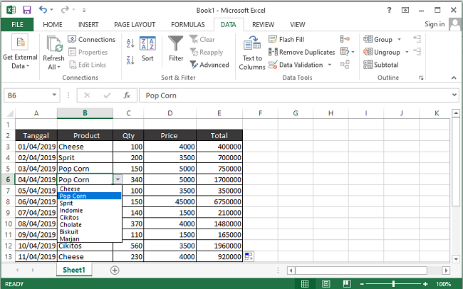
The first step to creating a drop-down list in Excel is to select the cell where you want the drop-down to appear. Then, navigate to the Data tab in the ribbon, and click on the Data Validation button. In the resulting dialog box, select the Settings tab, and choose List from the Allow drop-down list.
Customizing a Dropdown List
Once you have created a basic drop-down list, you can customize it to meet your specific needs. One way to do this is by adding a title or label to the list, which can help users understand what the list represents and how to use it. To add a title or label, simply enter the text into the cell above or below the drop-down list cell, and format the text as desired.
You can also add more options to the drop-down list by editing the list itself. To do this, select the cell with the drop-down list, and click on the Data Validation button again. In the resulting dialog box, select List from the Allow drop-down list, and then enter the new options into the Source box, separated by commas.
Creating a Dynamic Dropdown List
If you need to create a drop-down list that will change based on certain inputs, you can create a dynamic dropdown list. This can be helpful when you have a large data set with many variables, and you don’t want to manually update the list every time the data changes. To create a dynamic drop-down list, you will need to use a combination of Excel functions and data validation rules.
Start by setting up your data in a table with a consistent structure. Each column should represent a variable, and each row should represent an individual data point. Then, use the OFFSET function to create a dynamic named range that will adjust based on the selected variable. Finally, use the data validation feature to link the dynamic named range to the drop-down list cell, so that the list updates automatically based on the variable selection.
FAQ
How do I delete a drop-down list in Excel?
To delete a drop-down list in Excel, select the cell with the list, and then click on the Data Validation button in the Data tab of the ribbon. In the resulting dialog box, go to the Settings tab, and select No Validation from the Allow drop-down list. Click OK, and the drop-down list will be removed from the cell.
Can I use images in my drop-down list?
Excel does not support images in drop-down lists, but you can simulate the effect by using conditional formatting. To do this, create a range of cells with images or icons that correspond to the drop-down list options. Then, create a data validation rule that refers to the corresponding text values for each image. Finally, apply a conditional formatting rule to the drop-down list cell that displays the appropriate image based on the selected value.
Video Tutorial
For a comprehensive overview of creating drop-down lists in Excel, check out this video tutorial:


