Excel is a very powerful spreadsheet software that allows people to easily organize and analyze data. One of the useful features of Excel is the Freeze Panes option that allows you to keep certain rows and columns visible while scrolling through the rest of the data. In this article, we will explore how to use the Freeze Panes option in Excel.
Cara Freeze Excel Untuk Membekukan Baris & Kolom Supaya Tidak
The Freeze Panes option in Excel is used to keep certain rows and columns fixed while scrolling through the rest of the data. This is useful when you are working with a large data set and want to keep the column or row headings visible at all times. Here’s how to use the Freeze Panes option:
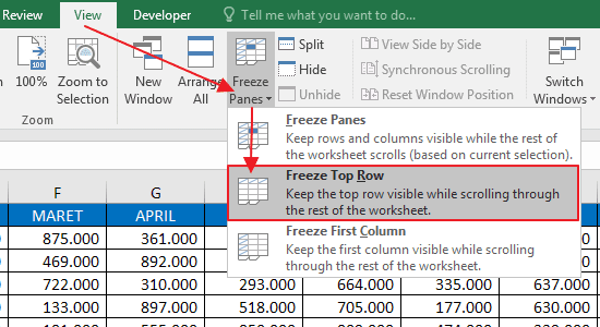
- Select the cell below the row that you want to freeze. For example, if you want to freeze the first row, select the cell in the second row.
- Click on the View tab in the Excel ribbon.
- Click on the Freeze Panes button in the Window group.
- Select either Freeze Panes or Freeze Top Row, depending on whether you want to freeze the selected row or column.
To unfreeze the panes, simply click on the Freeze Panes button again and select the Unfreeze Panes option.
Cara Membuat Freeze pada Excel untuk Kolom dan Baris
The Freeze Panes option in Excel can be used to freeze both rows and columns at the same time. Here’s how to use this option:
- Select the cell below the row and to the right of the column that you want to freeze. For example, if you want to freeze the first row and column, select the cell in the second row and second column.
- Click on the View tab in the Excel ribbon.
- Click on the Freeze Panes button in the Window group.
- Select the Freeze Panes option.
To unfreeze the panes, simply click on the Freeze Panes button again and select the Unfreeze Panes option.
FAQ
What is the difference between Freeze Panes and Split Panes?
The Freeze Panes option in Excel keeps certain rows and columns fixed while scrolling through the rest of the data. On the other hand, the Split Panes option is used to divide the worksheet into multiple panes so that you can scroll through each pane independently. You can access the Split Panes option by clicking on the View tab in the Excel ribbon and selecting the Split option in the Window group.
Can I Freeze Panes on multiple worksheets in Excel?
Yes, you can freeze panes on multiple worksheets in Excel. Simply select the worksheet where you want to freeze panes, and then follow the steps mentioned above to freeze the panes. Repeat this process for each worksheet where you want to freeze panes.
Video Tutorial
The Freeze Panes option in Excel is a useful feature that allows you to keep certain rows and columns fixed while scrolling through the rest of the data. This can be helpful when you are working with a large data set and want to keep the column or row headings visible at all times. By following the steps mentioned above, you can easily freeze panes in Excel and improve your productivity.

