Excel is an essential tool for businesses and individuals alike. Its many functions allow us to analyze and interpret data quickly and easily. One such function is the COUNTIF function, which we will explore in this article. We will also discuss the RANK function and the DOLLAR function, two other important functions in Excel.
What is the COUNTIF Function?
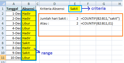
The COUNTIF function is used to count the number of cells in a range that meet a certain criteria. This criteria can be a specific value, a range of values, or even a text string. The syntax for the COUNTIF function is as follows:
=COUNTIF(range,criteria)
Here, range refers to the range of cells that you want to count, and criteria refers to the criteria that you want to use to count the cells. Let’s explore a few examples to better understand how the COUNTIF function works.
Example 1: Counting Cells with a Specific Value
Let’s say that we have a list of sales data, and we want to count the number of sales that were greater than $1000. We can use the COUNTIF function to do this. First, we need to select the range of cells that contains the sales data:
Next, we need to specify the criteria that we want to use to count the cells. In this case, our criteria is that the sales must be greater than $1000. We can enter this criteria directly into the formula:
=COUNTIF(B2:B11,">1000")
The result of this formula is 4, since there are 4 sales that were greater than $1000:
Example 2: Counting Cells with a Text String
Let’s say that we have a list of product names, and we want to count the number of products that contain the word “phone”. We can use the COUNTIF function to do this. First, we need to select the range of cells that contains the product names:
Next, we need to specify the criteria that we want to use to count the cells. In this case, our criteria is that the product names must contain the word “phone”. We can use the wildcard character (*) to represent any number of characters before or after the word “phone”:
=COUNTIF(B2:B11,"*phone*")
The result of this formula is 3, since there are 3 products that contain the word “phone”:
What is the RANK Function?
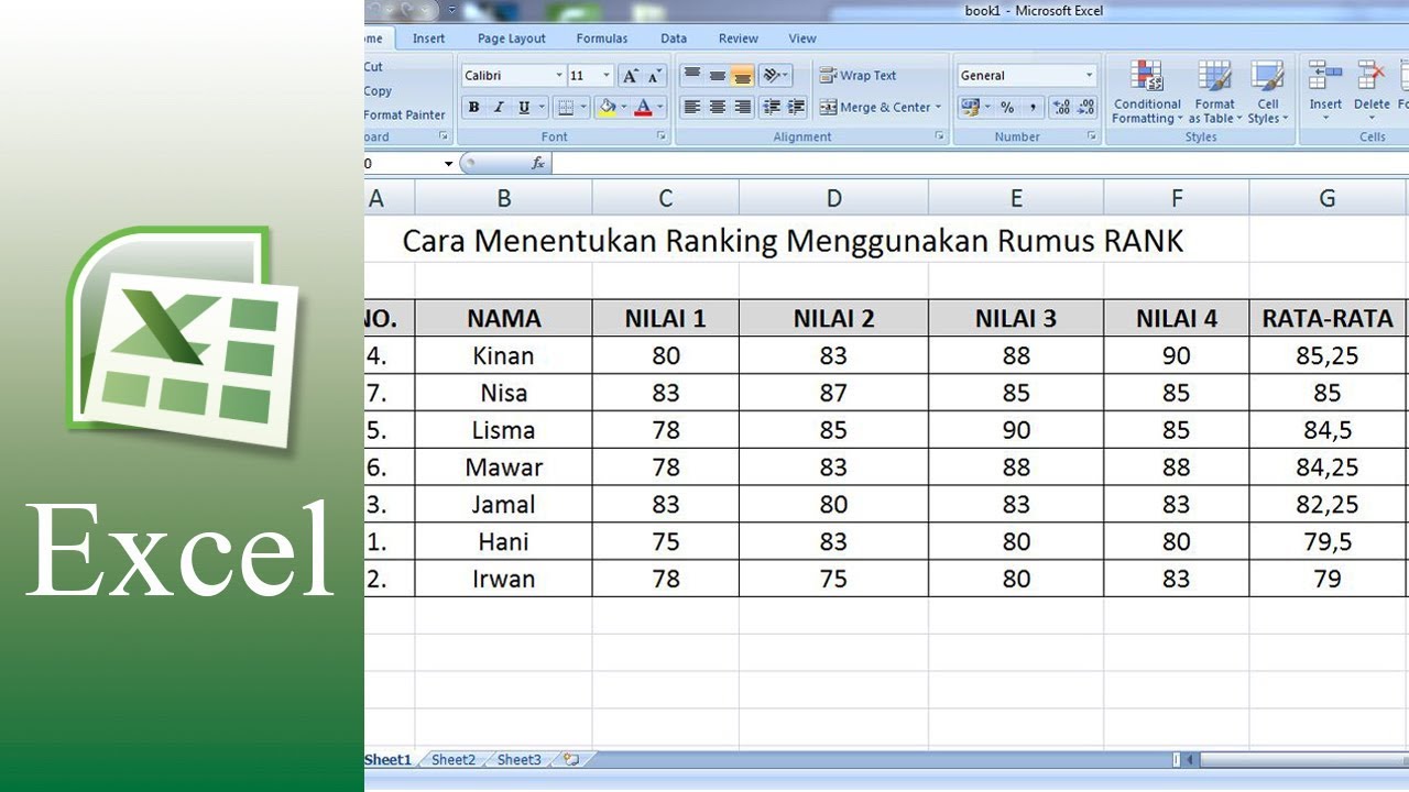
The RANK function is used to determine the rank of a value in a list of values. This can be useful when you want to know where a particular value falls in a list, or when you want to rank a list of values based on their importance or priority. The syntax for the RANK function is as follows:
=RANK(number,ref,order)
Here, number refers to the value that you want to rank, ref refers to the range of cells that contains the values that you want to rank, and order specifies whether you want to rank the values in ascending or descending order (1 for ascending, 0 or omitted for descending). Let’s explore an example to better understand how the RANK function works.
Example 1: Ranking a List of Values
Let’s say that we have a list of test scores, and we want to rank each score based on its position in the list. We can use the RANK function to do this. First, we need to select the range of cells that contains the test scores:
Next, we need to specify the value that we want to rank. In this case, we’ll rank each test score individually, so we’ll use a reference to each cell in the range:
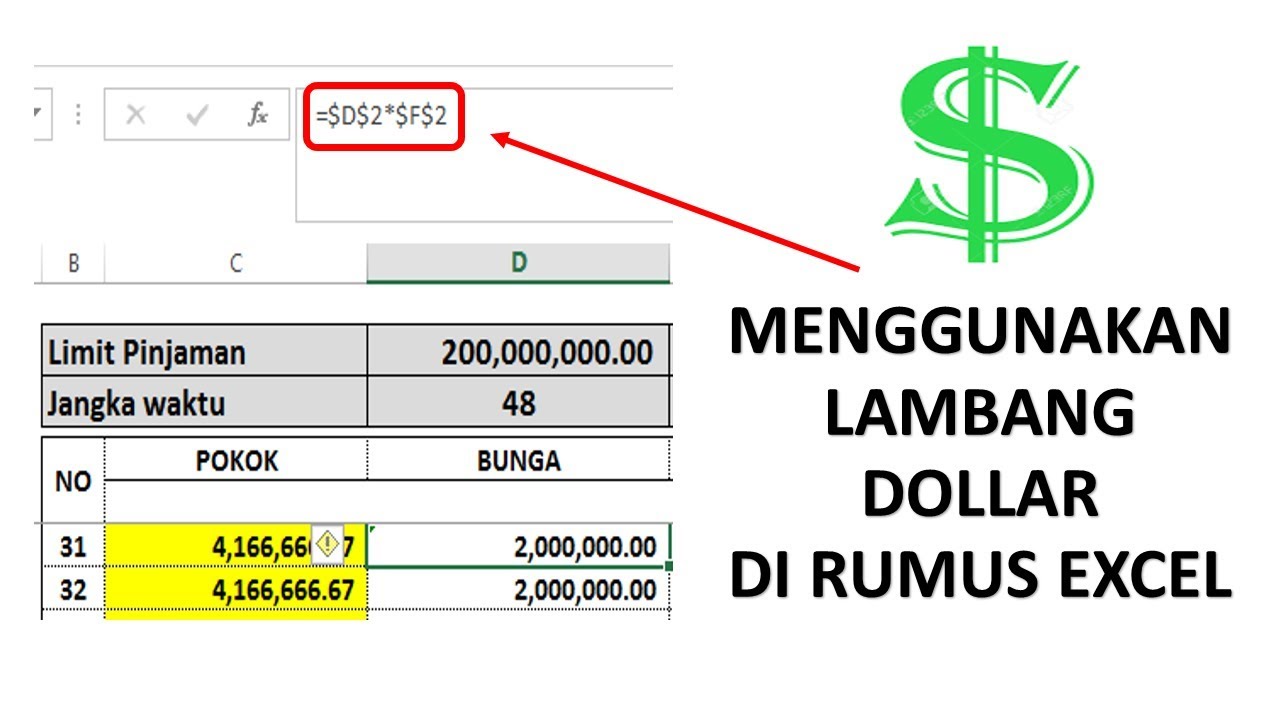
=RANK(B2,$B$2:$B$11,0)
The result of this formula is the rank of the test score in the list. For example, the first test score has a rank of 8, since it is the 8th highest score in the list:
What is the DOLLAR Function?
The DOLLAR function is used to format a number as currency, using the currency symbol and the specified number of decimal places. This can be useful when you want to present financial data in a clear and concise manner. The syntax for the DOLLAR function is as follows:
=DOLLAR(number,decimal_places)
Here, number refers to the value that you want to format as currency, and decimal_places specifies the number of decimal places that you want to display. Let’s explore an example to better understand how the DOLLAR function works.
Example 1: Formatting a Number as Currency
Let’s say that we have a list of sales data, and we want to format each sale as currency. We can use the DOLLAR function to do this. First, we need to select the range of cells that contains the sales data:
Next, we need to use the DOLLAR function to format each sale as currency. We’ll use a reference to each cell in the range for the number argument, and we’ll specify 2 decimal places for the decimal_places argument:
=DOLLAR(B2,2)
The result of this formula is the sale formatted as currency. For example, the first sale is $2250.00:
FAQ
1. Can the COUNTIF function be used with multiple criteria?
Yes, the COUNTIF function can be used with multiple criteria using the SUMPRODUCT function. For example, let’s say that we have a list of salespeople and their sales data, and we want to count the number of sales that were made by John in January. We can use the following formula:
=SUMPRODUCT((A2:A11="John")*(MONTH(B2:B11)=1))
This formula counts the number of cells where the value in column A is “John” and the month of the sale (extracted using the MONTH function) is January.
2. Can the RANK function be used to rank values based on multiple columns?
Yes, the RANK function can be used to rank values based on multiple columns using the CONCATENATE function. For example, let’s say that we have a list of employees and their sales data, and we want to rank each employee based on their total sales. We can use the following formula:
=RANK(CONCATENATE(B2,C2),$B$2:$B$11+$C$2:$C$11,0)
This formula ranks each employee based on their total sales, which is calculated by adding their sales in column B to their sales in column C.
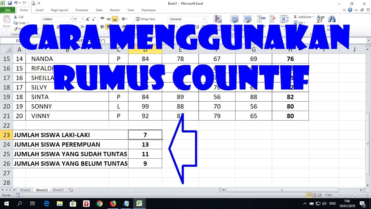
VIDEO: Cara menggunakan rumus countif di excel
If you’re still not sure how to use the COUNTIF function in Excel, check out this video tutorial:
Hopefully, this article has provided you with a better understanding of the COUNTIF, RANK, and DOLLAR functions in Excel. These functions can be incredibly useful when working with data, and can save you time and effort when analyzing and interpreting data.


