CARA MENYAMAKAN LEBAR KOLOM DI EXCEL

Have you ever struggled with aligning rows and columns, making data look neat and presentable in Excel? Fear not, as we have some easy solutions to help you out.

1. Automatically adjust row height and column width

One of the most common issues faced while creating an Excel sheet is the inconsistent size of columns and rows. This can make it difficult to read the data and can also look unprofessional.

Thankfully, Excel has a feature that allows you to automatically adjust the row height and column width to fit the content. Here’s how:

1. Select the row or column that you want to adjust.
2. Double-click on the line between the row or column header.
3. The row height or column width will now adjust to fit the content within it.

Excel also has another feature that allows you to adjust multiple rows or columns at once. Here’s how:

1. Select the rows or columns that you want to adjust.
2. Right-click on the selected rows or columns.
3. Click on “AutoFit” in the context menu.
4. The selected rows or columns will now be adjusted to fit the content.

2. Matching data in Excel

Another common issue faced while working with Excel is matching data from different sheets or workbooks. This can be especially difficult if you have a large dataset with numerous entries.

Thankfully, Excel has a useful function – VLOOKUP – which can help you match data easily. Here’s how:

1. Select the cell in which you want to enter the matched data.
2. Type the formula =VLOOKUP(lookup_value, table_array, col_index_num, range_lookup)
3. Replace lookup_value with the cell address or value that you want to match.
4. Replace table_array with the range of cells that you want to search for the match.
5. Replace col_index_num with the column number in the table_array that contains the data you want to retrieve.
6. Replace range_lookup with True or False depending on whether you want an exact match or an approximate one.
7. Press Control + Shift + Enter to complete the formula.

FAQs

1. What if I want to adjust the row height or column width to a specific value?

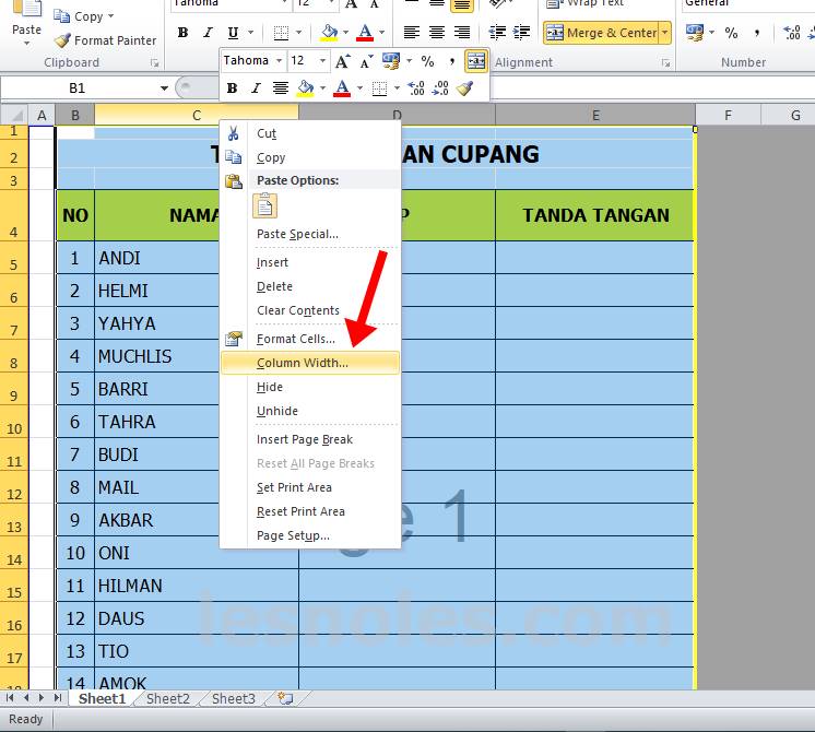
If you want to adjust the row height or column width to a specific value, you can do so by following these steps:

1. Select the row or column that you want to adjust.
2. Right-click on the selected row or column.
3. Click on “Row height” or “Column width” in the context menu.
4. Enter the value you want to adjust it to.
5. Click OK.

2. Can I use VLOOKUP to match data horizontally?

Yes. You can use HLOOKUP function to match data horizontally. Just replace VLOOKUP with HLOOKUP in the formula.

So, that’s how you can adjust the row height and column width in Excel, and match data from different sheets using VLOOKUP.

Here’s a video tutorial on how you can use VLOOKUP:

Now that you know these simple Excel hacks, creating and managing data will be a breeze!