I recently learned about some helpful tips for using Microsoft Excel, and I wanted to share them with you! Below are some of the techniques I found to be particularly useful:
Creating Dropdown Lists in Excel
Have you ever wanted to provide a list of options for data entry in Excel? One way to accomplish this is by creating a dropdown list.
Begin by selecting the cell(s) where you want the dropdown list to appear. Then, go to the “Data” tab in the Excel ribbon and select “Data Validation.” Under “Allow,” choose “List.” In the “Source” field, type the list of options separated by commas, or select the range containing the options.
Now, when you click on the cell(s), a dropdown arrow will appear, allowing you to choose from the list of options. This is a great way to ensure consistency in your data entry!
Creating Tables in Excel
If you frequently work with large amounts of data in Excel, tables can be a helpful tool for organization and analysis.
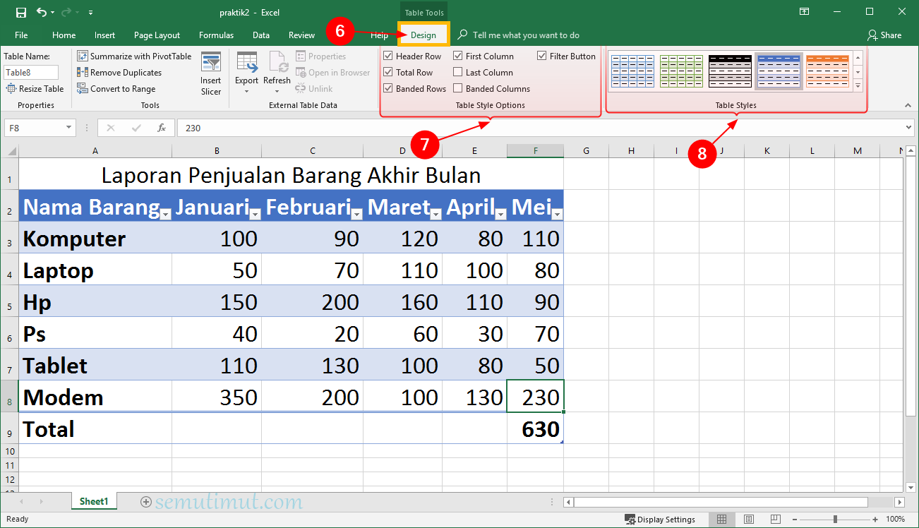
To create a table, first select your data range. Then, go to the “Insert” tab in the Excel ribbon and select “Table.” Make sure the “My table has headers” checkbox is selected if your data has column headers. Excel will automatically format the table with alternating row colors and filter arrows for each column header.
With a table, you can easily filter, sort, and analyze your data. Plus, any formulas, charts, or pivot tables you create based on a table will automatically update as you add or modify the data.
Using Percentages in Excel
If you need to calculate percentages in Excel, there are a few different methods you can use depending on your needs.
For example, to find the percentage of one cell relative to another cell, you can use a formula like this:
= (cell1/cell2) * 100
This will give you the percentage as a whole number. If you want to include the percent symbol, you can add it to the end of the formula like this:
= (cell1/cell2) * 100 & “%”
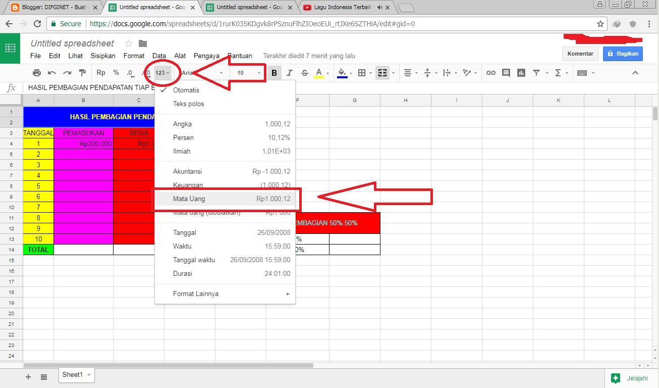
Alternatively, you can use Excel’s built-in percentage formatting to display a number as a percentage. Just select the cell(s) you want to format, go to the “Home” tab in the Excel ribbon, and choose the “Percent Style” button.
Creating Colorful Tables in Excel
While Excel’s default table formatting is useful, you may want to customize the colors to match your branding or make your data more aesthetically pleasing.
To create a colorful table, select your data range and go to the “Home” tab in the Excel ribbon. Choose the “Format as Table” button and select a table style with the “Table Styles” dropdown. Then, select “New Table Style” at the bottom of the dropdown, and customize the colors, font, and effects to your preference.
You can also create conditional formatting rules to highlight certain cells based on their values. For example, you could highlight any cells with a value above a certain threshold in green, and any cells with a value below the threshold in red.
FAQs
1. How can I sum a column of numbers in Excel?
To sum a column of numbers in Excel, you can use the “SUM” function. Simply select the cell where you want the sum to appear, type “=SUM(” and then select the range of cells you want to add. For example, if you wanted to sum the values in cells A1 through A5, you would type “=SUM(A1:A5)” and press Enter.
2. Can I create charts and graphs based on my Excel data?
Yes! Excel has a variety of chart and graph types you can use to visualize your data. Simply select the data you want to graph, go to the “Insert” tab in the Excel ribbon, and choose a chart type from the “Charts” dropdown. You can then customize the chart’s appearance and format the data labels, titles, and axis labels to your preference.
Video Tutorial
I hope these tips have been helpful in improving your Microsoft Excel skills. If you have any other tips or questions, feel free to share them in the comments!


