Excel is a powerful tool for organizing and analyzing data. But did you know that you can also add color to your Excel spreadsheets to make them more visually appealing and easy to read? In this article, we will explore different ways to add color to your Excel sheets. Whether you want to highlight specific data or create a colorful chart, we’ve got you covered.
Method 1: Using Conditional Formatting to Highlight Data
Conditional formatting is a feature in Excel that allows you to automatically apply formatting to cells based on their content. This can be a useful tool for highlighting specific data or trends in your spreadsheet.
To use conditional formatting, first select the range of cells that you want to apply the formatting to. Then, click on the “Conditional Formatting” button in the “Home” tab of the Excel ribbon. You will see a list of different formatting options, such as “Highlight Cell Rules” and “Color Scales”.
One common use of conditional formatting is to highlight cells that meet certain criteria. For example, you may want to highlight all cells that contain a value greater than 100. To do this, select the cells that you want to apply the formatting to, click on “Conditional Formatting” > “Highlight Cell Rules” > “Greater Than”. Then, enter the value that you want to use as the threshold (in this case, 100) and choose a formatting option (e.g. green fill color).
Method 2: Adding Color to Charts
Charts can be a great way to display data visually. However, charts can sometimes be difficult to read if they are too plain or if there are too many data points. Adding color to your charts can help to make them more visually appealing and easier to understand.
To add color to your chart, first select the chart that you want to modify. Then, click on any of the chart elements (e.g. bars, axes, legend) to reveal the “Format” tab in the Excel ribbon. From there, you can choose different fill colors, border colors, and other formatting options for each element.
Another way to add color to your charts is to use a chart style. Chart styles are pre-defined sets of formatting options that can be applied to your chart with just a few clicks. To apply a chart style, select your chart and click on the “Chart Styles” button in the “Design” tab of the Excel ribbon. You will see a variety of different chart styles that you can choose from.
Method 3: Coloring Rows and Columns
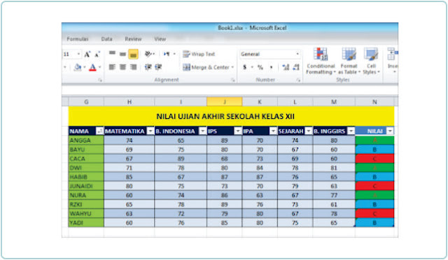
If you have a lot of data in your spreadsheet, it can be difficult to keep track of which row or column you are looking at. Coloring specific rows or columns can help to make your spreadsheet easier to read and navigate.
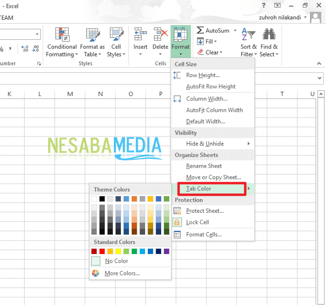
To color a row or column, first select the cells that you want to apply the formatting to. Then, click on the “Format” button in the “Home” tab of the Excel ribbon and choose “Format Cells”. In the “Format Cells” dialog box, select the “Fill” tab and choose a fill color for your cells.
Another way to color rows and columns is to use a shading feature in Excel. Shading allows you to apply a gradient color effect to your cells, which can make your spreadsheet more visually interesting. To apply shading, select the cells that you want to apply the formatting to, click on the “Format” button, and choose “Shading”.
FAQ
1. Can I change the default background color in Excel?
Yes, you can change the default background color in Excel. To do this, click on the “Page Layout” tab in the Excel ribbon, click on “Page Color”, and choose a new background color for your spreadsheet. This will change the default background color for all new workbooks that you create.
2. Can I save a list of custom color swatches in Excel?
Yes, you can save a list of custom color swatches in Excel. To do this, click on the “File” tab in the Excel ribbon, click on “Options”, and select the “Save” category. Then, click on the “Colors” dropdown menu and choose “Custom Colors”. From there, you can create a list of up to 16 custom color swatches that you can use in your spreadsheets.
Conclusion
Adding color to your Excel spreadsheets can make them more visually appealing and easier to read. Whether you want to highlight specific data or create a colorful chart, Excel offers a variety of tools to help you add color to your spreadsheets. Try out different methods and see which ones work best for you.
For more Excel tips and tricks, be sure to check out our video tutorial on adding color to your spreadsheets:


